Catastrophic cubic crash course

I’m happy to say that my advisor Ronen Eldan and I somewhat recently uploaded a paper to the arXiv under the title “Concentration on the Boolean hypercube via pathwise stochastic analysis” (https://arxiv.org/abs/1909.12067), wherein we prove inequalities on the Boolean hypercube using a cool continuous-time random process.

That’s quite a mouthful, I know, and quite unfortunately, Boolean analysis is not a standard part of any math curriculum that I know of, be it at the undergraduate, high school, or kindergarten level. In this post I explain a bit about what Boolean functions are and what sort of games you can play with them; a sort of catastrophic cubic crash course, if you will. The next post will talk about our actual result.

For your Boolean convenience, here is a small table of contents.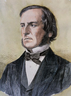

1. Boolean functions
2. Inequalities
3. Fourier for all
4. Hypercontractivity
5. Proving KKL

George Boole. Luckily for him, he would never dream of our stochastic atrocities.

Boolean functions

A Boolean function is a function which takes as input a vector of bits and outputs a single bit. That is, it’s just a function .

That’s it! Being so simple, Boolean functions can represent many things from many different disciplines, and it’s no wonder that they appear everywhere you look (though, as they say, what you see depends on what you are looking for, and this is especially true for mathematicians). To name a few examples:

• Social choice: A single bit can represent the opinion of a voting-age citizen concerning some political matter, e.g whether or not Earth should break from the Intergalactic Federation (Earthxit). The vector then represents the opinion of all citizens, and a Boolean function represents some way of deciding how to act based on those opinions. There are many ways to do this, as can be seen by the diversity of different voting schemes in the different countries of the world. For most of you, I suppose, the most natural way to aggregate the opinions is via the majority function, which outputs if and outputs if (i.e outputs if the majority of the inputs are and vice versa). For others, perhaps a more natural option is the dictator function, which just outputs for some index , corresponding to the idea that only the opinion of person matters.

  

• Algorithms: A very large portion of theoretical computer science and algorithms deals with concrete questions of the form “given some data structure, how do I know if it satisfies some property?”. For example, given a graph on vertices, does it contain a Hamiltonian path? Is it a tree? Does it contain a clique of size ? Is it 4 colorable? Is it isomorphic to some other graph? Is it planar? And many more. Now, a graph on vertices has a maximum of potential edges, and it is completely described by stating which of those edges appear, and which don’t. So a graph can be identified with a vector where each bit corresponds to some possible edge: if the edge is in the graph, and if it is not. Thus, each “graph property” you can think of gives rise to a Boolean function.

  For the connoisseur: Of course, the same is true not only for graphs; any Turing machine (which halts) gives a function on bits. But I’d like to stay away from the stratosphere, since if we keep things too abstract we lose sight of the road and of practical theorems. Graph theory and graph algorithm-related questions, as history has shown, provide a good supply of Boolean functions to study.

  

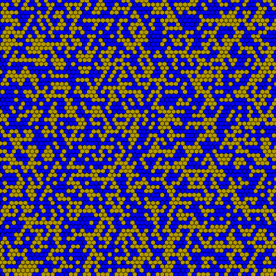
  Does this graph contain a clique of size 10?

• Percolation: Similarly related to the idea of “graph properties” but totally deserving an entry of its own is the percolation function. In this example, you start with a square which is divided into hexagons. Each hexagon is colored either blue or yellow, and so can be described by a single bit . The percolation function returns if there is a path of yellow hexagons from the left edge of the square to the right edge, and otherwise. The quest to understand percolation has driven forward much of the theory of Boolean functions and their properties, as is explained in the aptly named informative book “Noise sensitivity of Boolean functions and percolation”.

  

  Is there a left-to-right crossing of yellow hexagons?

• Combinatorics: A favorite pastime of mathematical combinators is to take an -element set , and ask all sorts of questions about how its different subsets interact with each other, such as “what is the largest possible family of subsets of so that no set contains the other?“. As it turns out, a family of subsets of can actually be viewed as a Boolean function, in the following way. Each represents a subset of , with if element number is in the subset and otherwise. A family of subsets then gives rise to a Boolean function , with if the subset represented by is in .
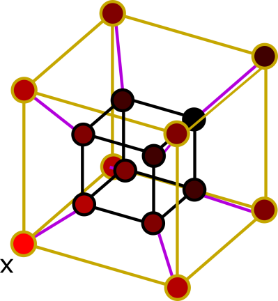
• And many more: There are a myriad other examples and uses. In fact, Boolean functions have already had a spotlight in this very blog, when I investigated random walks on the hypercube. Indeed, there are just too many to list. But that shouldn’t stop you from trying; as the saying goes, “The world is your oyster, and Boolean functions are the pearl”.

Inequalities

Mathematicians, being what they are, usually don’t care about any particular Boolean function and how to compute it, but rather are interested in general properties of Boolean functions, and how different properties relate to each other. And mathematicians, being what they are, have devised a fairly long list of properties and inequalities between them.

One of the central quantities of a Boolean function is its influence, which is a measure of how important each individual bit is to determining the value of the function . The definition is this:

Definition: Pick uniformly at random among all possible vectors. The influence of bit number on function , denoted , is the probability that changes its value when you flip the -th bit:

The dictator function shows well the purpose of this definition. For any input, flipping the -th bit always changes the output, so the influence of the dictating bit is , while flipping any other bit does nothing whatsoever to the output, so the influence of the rest of the puny bits is . Figuring out the influence of different bits for different functions is a fun game for the whole family. For some functions (such as majority), it is relatively easy; for others (such as percolation), you’re going to have to sweat a little.

The definition of influence uses elementary probability, and this is very common in the analysis of Boolean functions. For example, when faced with a new Boolean function, one of the very first questions you will ask is “is it balanced?”, meaning, does it output as often as it outputs ? You can quantify the bias of a function as

This will be if outputs as often as it outputs , but nonzero otherwise. Since there are possible values of to go through, the sum can potentially be as large as , and to be able to compare functions for different values, we usually use a normalized bias, whose range is in :

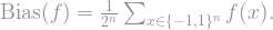
Ah, but now this already has a probabilistic flavor, since is exactly the probability of picking any particular vector uniformly at random. The normalized bias can then be written as an expectation:

This sort of thing is so popular that we will often just write and be done with it. The probabilistic notation conveniently leads to the “variance” of a function, which is defined exactly like in probability:

Since , a function which is balanced (i.e has ) will always have variance . However, the more biased a function is towards either or , the smaller its variance.

Having defined two different quantities, the first thing that a mathematician does is try to compare them. Here is a theorem, called the “Poincaré inequality”, which is true for all Boolean functions:

Theorem:

Amazing, isn’t it? Poincaré’s inequality is just the first among many inequalities which try to relate between the variance of a function and its influences. Among the Booleaners, it’s actually considered a rather weak inequality, and is not tight for any interesting function, really. For example, if you did your homework with your family above, then you probably discovered that for the majority function, every bit has influence on the order of . This means that the term on the right hand side is of size about , while the term on the left hand side is a mere puny ! That’s a lot of slack.

A much more powerful (indeed, revolutionary) inequality is the one proven by Kahn, Kalai and Linial in 1988.

Theorem (KKL): Let be the largest influence of , i.e . Then

Here is some fixed constant, and we don’t really care about its value.

We are usually interested in the behavior of these types of theorems when the number of bits goes to infinity (otherwise, there is only a finite number of functions, and so only a finite number of different values that and can get, and we can always pick to be large enough so that the theorem trivially holds). And when the number of bits goes to infinity, we also want the maximum influence to go to , for quite the same reason. But as , the factor becomes very small! so for all interesting cases, the quantity in the right hand side of the KKL inequality is smaller than that of the right hand side of the Poincaré inequality; the KKL theorem is indeed the stronger of the two. It is still not tight for the majority function, but there are other interesting functions for which it is tight.

Fourier for all

The KKL inequality is the industry-standard, go-to inequality for Boolean functions; efficient, dependable, and quite importantly, analysable. Its most common proof showcases the mathematical gizmos and gadgets used in Boolean analysis. Let’s take a peek at them.

At the core of everything Boolean lies the Fourier decomposition: Every function can be written as a multivariate polynomial:

where the term is called the “Fourier coefficient” of the set . Here are two ways to see why this is true:

1. The brute force way: One way to “compute” the function is to go over all possible vectors , and ask, “is equal to ? If so, then return !” Mathematically, this amounts to writing as the sum over the indicators of its inputs:

   

   where is the function which returns when and otherwise. Luckily, this function can be written as a polynomial in the entries of : For every bit , the expression is if (i.e they have the same sign) and if (i.e they have different signs). Since we need every bit to agree with every bit , we just have

   

   Plugging this into the sum over indicators and summing over possible monomials instead of over possible values then gives the decomposition. Note that some of the may be .
2. The elegant way: Like everything elegant in the world, this way uses linear algebra. For a set , denote ; this is called the “character” of . A simple calculation shows that for , the correlation between and vanishes:

   

   Thus the set of characters constitute a complete orthonormal basis under the scalar product , and so every function (being a member of the -dimensional linear space of all functions on ) can be written as a linear combination of characters . To obtain the coefficients of the combination, all you need to do is take a scalar product again:

   

The second, elegant way has a few advantages. First, if you took a functional analysis course in kindergarten, it makes you feel proud to finally see it applied in a nontrivial discrete system. Congratulations! Second (and perhaps arguably more important), the connection to classical functional analysis automatically gives us access to a vast repertoire of theorems and results about this decomposition. For example, we immediately know that the decomposition is unique, or that an equality known as “Parseval’s identity” holds:

By definition of the particular scalar product we use, , this actually gives

We can then write the expectation and variance of a function in terms of its Fourier coefficients: The expectation is just the coefficient of the empty set:

and using this fact and Parseval’s identity, the variance is

(since we subtract the expectation, we take the square of all coefficients except that of the empty set).

This is very neat; we have found a way to express the variance of a function using its Fourier coefficients. Perhaps, if the same thing can be done for the influences , we could compare directly between the two quantities and prove inequalities like Poincaré and KKL. For this, we use derivatives:

Definition: The -th derivative of a Boolean function , writen , is given by the difference of ‘s value when takes the value and :

The derivative function can take on three possible values: , if ‘s value changes when flipping bit , or if it remains unchanged. So the square of the derivative, , has value if flipping bit changes the output. Since is just the probability of this thing happening, the influence is equal to

Luckily, if we know the Fourier representation of , then we also know the Fourier representation of its derivative: You can differentiate each monomial separately, and find that

Again invoking Parseval’s identity,

If we sum over all indices , we’ll again get a sum involving the Fourier coefficients of , but now each coefficient will be multiplied by some factor: Each set appears once for each , so each Fourier coefficient is counted times. The empty set won’t be counted at all, of course. Thus

Congratulations! We have just proven Poincaré’s inequality: The variance had exactly the same form, but without the term multiplying each Fourier coefficient. But always, so the sum of influences is always larger than the variance. And, if your body is willing and your spirit is strong, you can even deduce from these representations for which functions the Poincaré inequality is actually an equality.

Hypercontractivity

Unfortunately, the KKL inequality requires more than basic manipulation of Fourier coefficients (indeed, it requires advanced manipulation of Fourier coefficients). The standard proof uses what is known as the “hypercontractive inequality”. Summed up in one cryptic sentence, this inequality tells you how different ways of sizing up a function (aka different norms) relate to each other when you smooth out the sharp features of the function (aka adding noise). Let’s see what all of that means.

One important way of studying the influences of a function is to see how it changes under noise. You can write entire books on this topic (indeed, people have), so I’ll just present the basics here.

First, what is noise? Suppose that is a point in the hypercube. A random vector is said to be -correlated with if each bit is obtained from by setting with probability , and setting with probability . In other words, is like , but each bit of has a chance of of being “rerandomized”, i.e has a chance of being uniform random. When , we just have , since the probability to be rerandomized is . When , then is just uniformly random, since the probability of being rerandomized is , and when is somewhere in between, then is somewhere in between; the larger the , the higher the probability that many bits of agree with the bits of . We often think of as a “noised version” of . This has a geometric interpretation: For small values, most of ‘s bits should be identical to those of , and so it is (physically) close to it in the hypercube.

The probability of getting a point y which is correlated with the lower-left corner is given by the color; the brighter the vertex, the higher the probability.

Using this definition of noise, we can look at a “smoothed out” version of , where instead of looking at , we look at where is a noised version of . This is called the noise operator.

Definition: The noise operator of , denoted , is defined as

where is -correlated with .

I say that this is “smoothed” out because what it does in effect is take weighted averages over all the values of , where larger weights are given to points close to , and smaller weights are given to points far away from (since there is a higher probability for to be close to than far). For , all the weights in the average are the same, and we just take a simple average of all the points in the hypercube, i.e is the constant function . For , we take the average of only one point, and . Another reason that that is is called “smoothed” is that whereas the original function takes values only in , the noised version takes values in the continuous interval . Smooth indeed 😎.

For the connoisseur: If you peek inside textbooks, you might see appear under the name “heat operator”. Indeed, you can imagine that a point in the hypercube is a hot body (say, a hot potato), while all the other vertices are cold (say, cold potatoes). Imagine also that vertices transfer heat to each other via conduction, and every vertex transfers heat equally to all its neighbors in proportion to the temperature difference. In this case, it turns out that the temperature at a vertex is proportional to the probability that , where is -correlated with .

It can sometimes be a bit hard to understand how behaves, but as usual, one way to study it is to see what it does to the Fourier coefficients. Since the expectation is linear, i.e , we can apply to each monomial in the Fourier decomposition of :

Luckily, the effect of on the monomial is relatively easy to understand: Since all the bits are independent, it’s just the product of on each individual , and each one of those is equal to

So all in all,

and if we know the Fourier coefficients of , then we know the Fourier coefficients of ! Namely,

This representation is very useful, and Booleanists learn it by heart from an early age.

While the noise operator certainly changes the values of , it does not change the expectation of , so if we take a sum of over all and a sum of over all , we get the same result. Of course, this does not hold for averages over other quantities derived from , for otherwise there would be no difference between and . For example, in general,

(since always and can be smaller than ). Many doors now open, and the mathematically-curious can wonder how expectations of quantities of relate to expectations of quantities of . One class of heavily-investigated such quantity is the -norm:

Definition: Let . For , the -norm of a function , denoted , is defined as

The -norm is important in many branches of analysis, and Boolean analysis is no exception. The friendliest norm you can find is the -norm: Its cheerful disposition arises mainly from Parseval’s inequality, from which we learn that

this connects the study of norms to the study of Fourier coefficients. Still, mathematicians and computer scientists do not take favorites, and apart from the -norm, other -norms are uniformly studied (if not loved). A bit of analysis using convexity can show the following inequality between norms: If , then

In other words, taking a larger only increases the size of the norm. To get a feel of why this is true, think of a function which outputs on a single input , and outputs on all the rest. The expectation will always be , but the root on the outside makes the norm larger for larger values of .

For the connoisseur: The keen-eyed among you will have noticed that the inequality between norms is exactly the opposite of norms for functions on (and general normed spaces); in those cases, we have for . The reason for this reversal is the introduction of the factor by the expectation for the Boolean case.

The inequality can be thought of as follows. As the name suggests, the -norms are “norms”, as in, they can be used to measure distance. The norm measures the “distance” of from the constant function , and the distance between two functions and is given by . The inequality is then equivalent to saying that the identity mapping between the space of all Boolean functions where distances are measured using the norm and the space of all Boolean functions where distances are measured using the norm is a contraction. More succinctly: The operator is a contraction.

With this notion in mind, we come to perhaps the most famous theorem in the study of norms of Boolean functions, the “Hypercontractive inequality”. This is a really fancy-sounding, sex-appealing name for a theorem which relates the norm of and the norm of its smoothed version, . It states that:

Theorem: For all ,

Since always, the subscript 2 is always larger than the subscript , which means that the inequality goes in the opposite direction of the “inequality of the contractive identity”. In other words: Although the -norm of is always larger than the -norm of , the inequality is reversed if we smooth out by amount of noise. In even other other words: The noise operator is a contraction! This is the origin of the overwhelming “hypercontractive”: The noise operator is so good at equalizing and reducing the norm of a function, that not only is it contracting in its original space (i.e ), but it is even a contraction when comparing to otherwise smaller norms!

When I just started learning about Boolean functions, I didn’t know what all the fuss was about. After all, it’s just another inequality. But if there’s one thing that the analysts are good at, it is squeezing seemingly obscure inequalities to their very last drop of sweet, theorem-proving juice. Let’s see how that works out for the KKL inequality.

Proving KKL

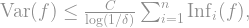
Armed with the hypercontractive inequality, proving KKL is as easy as a brisk walk in an -dimensional park; the elegant proof I present here is from the book on noise sensitivity. In essence, the proof uses the Fourier decomposition of to show that much of the contribution to the variance can be bounded by smoothed-out versions of the derivatives of . These smoothed-out versions can then be bounded using the hypercontractivity theorem. To save you some scrolling, here is the KKL inequality:

Theorem (KKL): Let be the largest influence of , i.e . Then

Assume for now that (we’ll show what happens when afterwards). We start the same way we proved the Poincaré inequality, by writing as a sum of Fourier coefficients:

What we did when proving the Poincaré was to multiply each summand in the right hand side by ; since , this only made the summands larger. When we did this, the right hand side was equal to the sum of influences, by the Fourier analysis we did before.

This time, we’ll do something similar, but use a trick before multiplying by : We pick some number (to be defined later) and divide the sum into two parts: All those which are smaller than , and all those which are larger:

For the first sum, we just multiply every summand by as usual. But for the second sum, since there, we actually multiply by ; this is still a number larger than , so we still only increase the size of the summands:

The second sum is certainly smaller than the sum of all influences, again by the Fourier expansion of the sum of influences that we saw above. So

To bound the first sum, we use another clever trick: We multiply each summand by and divide by ; this only makes each summand larger, since . We can also extend the sum to all , since that only adds more terms, and we arrive at the inequality

Here is where, at last, the heat operator and hypercontractivity come in. Recall what the heat operator does to the Fourier representation of a function: It adds a factor of to each Fourier coefficient. So if we look, for example, at the effect of on the derivative of in direction , we get

and the square of the -norm of this expression is, by Parseval’s identity, just the sum of square of coefficients:

The equations practically (but metaphorically) beg us to sum this expression over all indices ; if we do that, we’ll count each set as many times as there are indices in it (very similar to the calculation for the sum of influences), giving

All that remains is choose the very down-to-earth value , and we have a bound for our initial sum:

By the hypercontractivity theorem, the -norm of the smoothed is smaller than the -norm of the original function , so

But the -norm of the derivative to the power of is just the influence of the function , since the derivative is when there is a change in the function’s value and otherwise! And since every influence is bounded by by definition, we reach the final bound on the first sum:

When we put this together with the bound on the second sum, we get a nice bound on the variance:

All that remains is to choose a which will minimize the expression in the parenthesis. Notice that as increases, the term increases, but the term decreases. Typically, these types of expressions are minimized when both terms are equal, or at least, nearly equal. To do this, choose

with the logs in base 2. Upon plugging this into the first term, the -power vanishes, and we are left with . As for the second term, since we assumed way way up in the beginning of this section that , the factor doesn't really make much of a dent in the much larger term, and 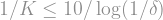. So all in all,

exactly as prophesied!

(And what if ? Well, in that case, , so in this case the KKL theorem is basically the Poincaré inequality in disguise, with a large constant in front of the influence term).

All in all, I think this is a nice proof. The choice is of course arbitrary; we could have chosen a different noise level, and gotten other constants in the various calculations. But the point remains the same: We found a suitable fixed noise level (or, “heating time”, if you think about as a heat operator) where we could safely bound the smoothed-out versions of the derivatives. In the next post I will talk about my advisor’s and my new work, which shows how finding a random noise level can help you prove even more powerful versions of KKL-like inequalities.