Random graphs: The duplicube graph + new paper on arXiv

Some mathematicians like probability, and some mathematicians like graphs, so it’s only natural that some mathematicians like probabilistic graphs. That is, they like to generate graphs at random, and then ask all sorts of questions about them: what are the features of a random graph? Will it be connected? Will it contain many triangles? Will it be possible to color it with colors without coloring two adjacent vertices in the same color? Will it bring me tenure? They may also check if the graphs can be used in order to prove other theorems, or if they can represent real-world networks in some way.

The answers to all these very interesting questions (interesting to some of us, anyway) depend very much on what we mean when we say that we “generate a random graph”. In fact, for the phrase “generate a random graph” to be meaningful, you must tell me the distribution’s probability law; that is, you must tell me, for each graph, what is the probability of obtaining it. Only then can we carry out the calculations.

There are many ways of choosing such a law; in this series of posts I will present the random graphs commonly found in mathematics and network theory, and demonstrate some of their properties.

And today, a bonus! Today’s random graph model was suggested by Itai Benjamini, and investigated by Itai, Yotam Dikstein, Maksim Zhukovskii and myself. I am happy to say that we have just uploaded a paper to the arXiv, titled “The duplicube graph – a hybrid of structure and randomness” (https://arxiv.org/abs/2211.06988) detailing our investigation.

---

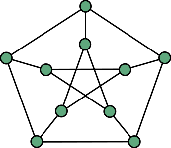
The whole thing is based on a simple operation, “duplimatching”, which goes like this. Suppose you already have some graph at hand:

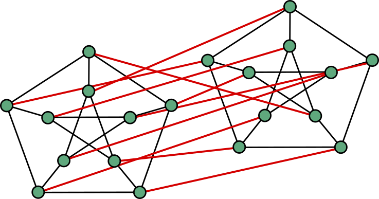
Now take two copies of this graph, and add a perfect bipartite matching between the two copies; in other words, you connect all the vertices of one copy to those of the other, so that each vertex is part of exactly one new edge. Like so:

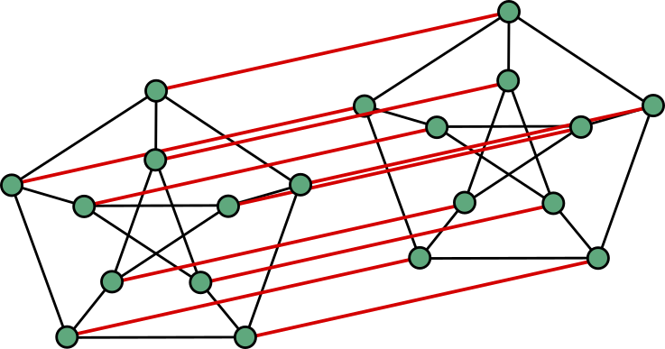
You now have a new graph with twice the number of vertices as you had before. Of course, this graph heavily depends on how you chose to match up the vertices of the two copies. The above example was generated randomly, but I could have also chosen to connect the vertices like so, giving much more sense and structure to the new graph:

Indeed, the above matching — the identity matching, basically — is very natural, and can easily be applied to every graph — you just connect each vertex to its own copy. However, since this is a post on random graphs, you probably already guessed that we will also be talking about random matchings. The simplest random matching is the uniform matching: if your original graph has vertices, it is a matching chosen with equal probability among all possible matchings. A way to construct it as follows: order the vertices of one copy, and connect them one by one to the other copy, each time choosing a vertex uniformly at random from all those that hadn’t been chosen yet.

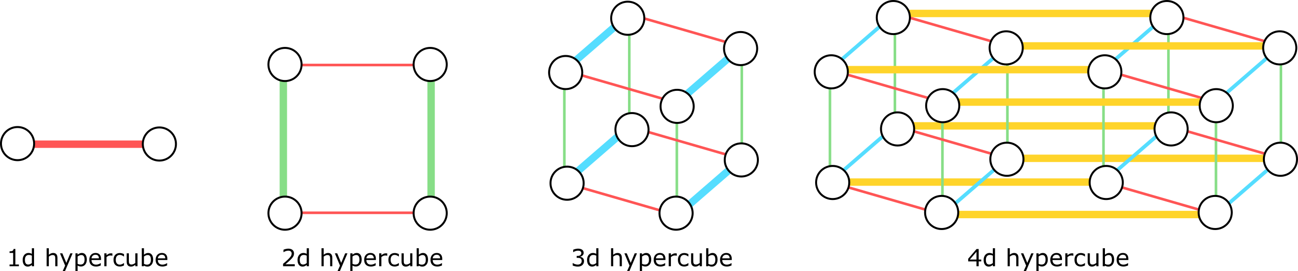
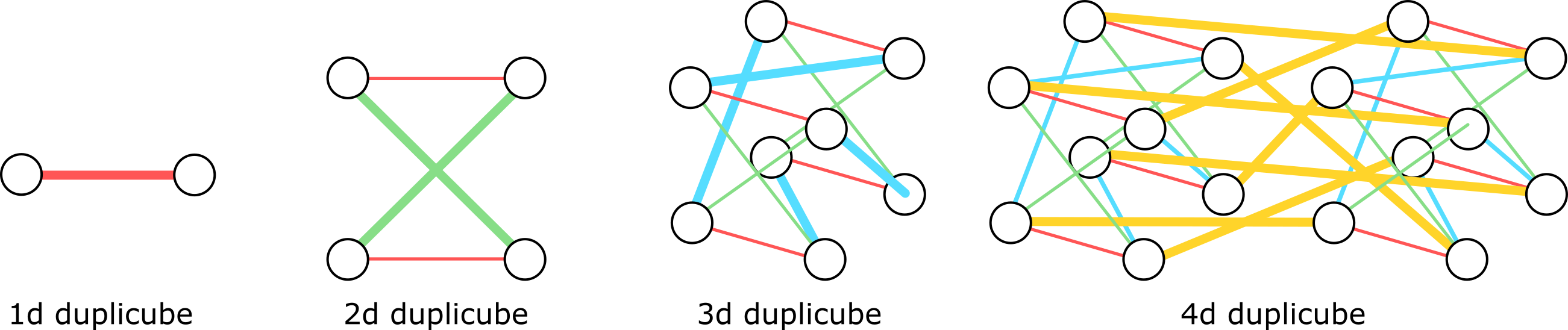
So that was the duplimatching operation. What then is the duplicube? It is just the repeated application of the duplimatching operation. You start with a single vertex, and, after iteratively applying the duplimatching operation times, get some graph on vertices, depending on which matchings you chose along the way.

If you love law and order and chose the identity matching every time, then after iterations you’d get the -dimensional hypercube, denoted , whose vertices are and whose edges connect two vertices if they differ in exactly one coordinate.

If you are entropically-inclined, however, and chose a random matching every time, then you’d get something else entirely. This is the random duplicube graph, which we denote here by .

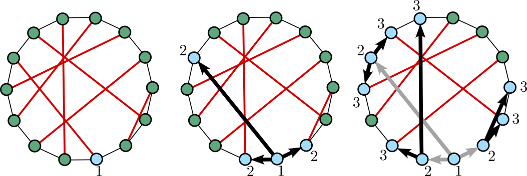
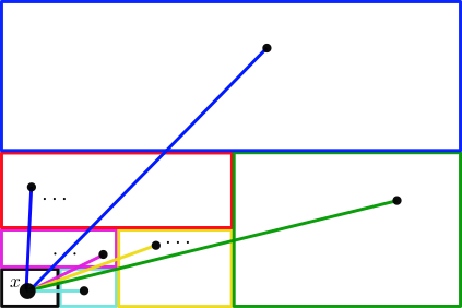
How do you make sense of this graph? As noted above, after iterations, you get a graph on vertices, and each vertex has degree exactly , so in total there are edges. These edges can be partitioned into perfect matchings on these vertices (as indicated by the colors in the above picture). These matchings are random, but not uniformly random among all possible matchings on vertices — the matchings that we chose very early on in the process are heavily duplicated. This gives a lot of dependence between the edges, and makes the duplicube a sort of “hybrid graph”. If it was just a union of independent, uniformly random matchings, then it would be very similar to a random -regular graph (which itself is very similar to a Erdős–Rényi random graph). But it is not — the matchings still remember some of the structure induced by the repeated duplicating operation, and so the graph, at least superficially, has something in common with the hypercube as well. This already makes it an interesting object to research: the aspiring mathematician can ask herself in what ways the duplicube is similar and different than these other famous models.

In this post we’ll talk about just two quantities of the duplicube — its diameter, and its eigenvalues. In the arXiv paper, we also have results on its vertex expansion and symmetries (or lack thereof), as well as a plethora of open questions and further directions.

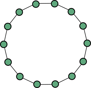
The diameter
The diameter of a graph is the largest distance between any two of its vertices (i.e. the length of the longest shortest path between any two vertices). As a warm up, what is the diameter of an -vertex cycle?

If and are two points on opposite sides of the cycle, then you need to take steps to get from one to the other. So the -vertex cycle has large diameter — proportional to the number of its vertices. On the other hand, for the hypercube , which has vertices, the diameter is only : if and are two points in the hypercube, then the distance between them is just the number of entries for which . This means that the hypercube is quickly navigable: its diameter is logarithmic in the number of vertices. In fact, it can be shown that if a graph has vertices, and the degree of every vertex is at most , then the smallest diameter it can have is of order ; (this bound is in fact attained, up to constant factor, by random -regular graphs). This means that the hypercube misses the smallest diameter possible by a factor of , which is really tiny compared to itself.

What about the duplicube, then? It too is an -regular graph on vertices. How does its diameter compare with that of the hypercube?

As a first result, we note that it is always smaller than that of the hypercube, i.e. its diameter is always at most . This can be proven by induction: suppose and are two vertices of the duplicube. If they are on the same “side” of the largest cut of the duplicube, then you only need at most steps to go from one to the other, where these steps are all contained in the same side. And if and are on different sides, then take one step from to its neighbor on ‘s side; now the distance between and is at most , so in total the distance between and is at most .

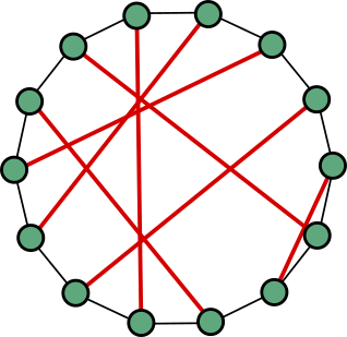
The immediate question that then comes to mind is: how much smaller can this diameter be? We already mentioned that it cannot be smaller than anyway, but can this bound actually be attained? A clue suggesting that the diameter can be quite small is given by the following cute result. Let’s look back at the -vertex cycle. This cycle has a very large diameter — proportional to the number of vertices. What happens if you add a uniformly-random matching to it, i.e. divide the vertices into random pairs and connect them together?

In a paper by Bollobás and Chung, it was shown that this reduces the diameter all the way down to (plus a tiny term, with high probability)! The addition of a single, completely random matching gives a logarithmic reduction in the diameter. Now, for the duplicube, the matchings aren’t random — even the “topmost” matching, the one added last which connects the two copies, is only a bipartite matching, and not a matching between all the vertices, while the matchings added at the beginning of the process have very little randomness in them. Still, we do add lots of matching, and it stands to reason that a significant reduction can be made. And, mathematics being overall reasonable, this is indeed the case:

Theorem: When the matchings are random, the diameter of satisfies

with high probability.

This does not match the best possible diameter, which is in fact attained up to a constant factor by random -regular graphs and has a in the denominator, but it is still an asymptotic improvement over the hypercube! And it is only an upper bound: we do not actually know what the real diameter is.

The way these results are often proved, is to show that for every two vertices and , there is, with high probability, a short path between them. And the way to do this, is to look at all the vertices reachable from by “short path length / 2” steps, and look at all the vertices reachable from by “short path length / 2” steps, and hope that these two sets are themselves connected by an edge. The distance between and is then bounded above by “short path length” (+1).

Bollobás and Chung do exactly this when they show that a cycle+matching has smaller diameter. They reason as follows. If you start at and look at all the vertices a single step away, you reveal three new vertices. Two of these are just going to be the original neighbors of , but one of them will be some random point on the cycle. Now look at where another step can take you. For the two vertices which were the original neighbors of , you again expand out to the sides of the cycle, but also gain two additional “random jumps”. Each time you do this “random jump”, it’s as if you gain new “seeds” from which to start expanding. So, repeating this process, the growth in the number of vertices you visit after such steps is almost exponential in . Why only “almost”? Because there is always a chance that the random jump ended up in a vertex which you already visited. However, Bollobás and Chung showed that if you only take a small number of steps (of order ), accidentally revisiting a vertex this way will only happen a very, very small number of times, so for all practical purposes, the growth is indeed exponential. This is, in essence, what gives you the diameter.

Alas, this argument could not be repeated as-is in the duplicube case, since, as mentioned before, the edges are not independent, nor uniform from each other. In the “cycle+matching” case, there were only two kinds of edges: those of the original cycle, and the “random jumps”. In the duplicube case, there are no “original” edges; rather, there are always different types of edges, each with their own independence properties. If you just say “let’s follow all the edges coming out of this set of vertices”, it’s very hard to keep track of when you discover new vertices, and when you jump back to vertices that you already visited, so it’s very hard (at least for us) to give good bounds on how large the set of vertices you reveal is.

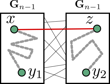
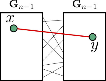
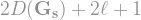
To overcome this, we used the hierarchical structure of the duplicube, in two ways. First, by the recursive construction of , we know that if you only follow “small generation edges”, i.e. edges that were added early on in the construction, then you can’t leave the large-scale structure that you are in. More concretely, here is an example. Suppose you start with some vertex , and look at the vertex that it’s connected to by the last matching. Then the vertices and are on two different copies of :

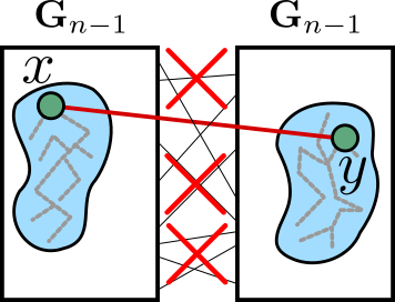
If we start recursively looking at the neighbors of and , but only adding neighbors which are connected by edges formed at earlier-generation matchings, then there is never any risk that the vertices revealed when starting with as the seed will connect to those revealed by starting with as the seed. In other words: once we make the jump , we never follow any more edges that cross the gap between the two copies of .

This reasoning can actually be recursively applied, where, if you follow along an edge generated by a -generation matching, you agree to only explore along lower-generation edges from that point on. This way, there will be no clashes at all, and you will never revisit the same vertex twice, allowing us to relatively-easily calculate the number of vertices we explore this way (the downside, of course, is that we may have missed lots of available vertices by ignoring so many edges, so the set of revealed vertices is definitely not as large as it could be). Thus, if we start at some vertex , we get a not-too-small set of vertices at distance at most from .

The second way we use the recursive construction of the duplicube is, well, by recursion. For , the duplicube contains copies of its young self, . We can therefore use induction, and rely on the fact that the diameter of is smaller than , so, starting from any vertex, taking steps will reveal at least new vertices. In other words, the ball of radius around any is of size at least . By looking at all the balls of this radius around every , we effectively multiply the size of by , giving us a new set which is already quite big. With this set, we finally use the standard argument: if it happens that and are connected, then there is a path of length between and . And almost by divine intervention, it is possible to tune the parameters and so that i) and are indeed connected with high probability, and ii) the length is smaller than .

Eigenvalues
The graph has vertices, and therefore it can be represented as a matrix , with if vertex is connected to vertex , and otherwise.

The adjacency matrix, being a symmetric matrix, has real eigenvalues, and mathematicians, acting naturally, like to study these eigenvalues. There are good reasons to do so, though; for example, the difference between the largest eigenvalue and the second largest tells you a whole lot about the edge-expansion, or about how quickly random walks mix on the graph, and these concepts have important, world-shaking consequences (if your world is small enough). It is not surprising then, that people know quite a lot about the eigenvalues of (the adjacency matrix of) various graphs, and this includes the hypercube and random regular graphs.

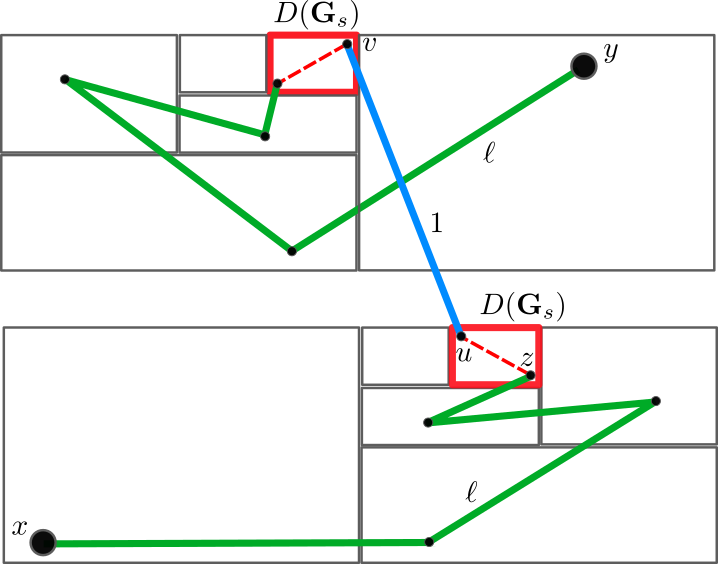
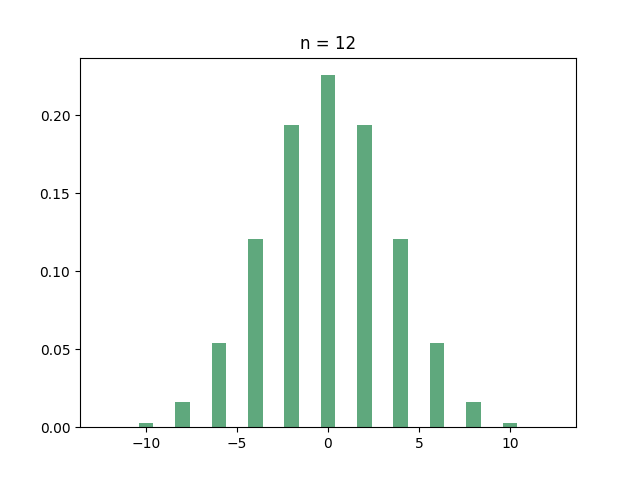
Let’s start with the hypercube. If you ask your computer to find out the eigenvalues of the hypercube, you’ll discover that many of them are identical. In fact, here is the histogram of the eigenvalues for several small values of :

If you have recurring nightmares from “Introduction to probability theory”, then you should immediately recognize the all-too-familiar shape of the binomial distribution. And this is indeed what’s going on:

Theorem: For every integer , the adjacency matrix of the hypercube has eigenvalue with multiplicity .

In what sense does this mean that the eigenvalues are “binomial”? Well, since there are eigenvalues, if you pick an eigenvalue uniformly at random then every eigenvalue has probability of of being picked. Since there are eigenvalues with the same value , the probability of picking is exactly the probability that a binomial random variable with trials and success probability has successes. In other words: if is a random eigenvalue of the hypercube, then

where are just independent Bernoulli random variables with success probability . Now, as we learned in kindergarten, by the central limit theorem, the sum of these random variables, when scaled by a factor of , converges in distribution to a standard Gaussian as . So the scaled eigenvalues of the hypercube have a limiting distribution! (warning: creating the adjacency matrix of the hypercube, diagonalizing it, choosing a random eigenvalue and then normalizing it is a very inefficient way of sampling a Gaussian).

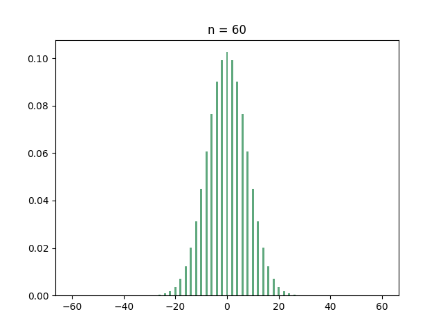
As it turns out, the eigenvalues of many random graphs also have a limiting distribution (in fact, this is common with many models of random matrices, of which the adjacency matrices of random graphs are just a specific case). For example, here is the (average) histogram of the eigenvalues for random -regular graphs with vertices:

If you are thinking, “This histogram does not look at all like the eigenvalues of the hypercube. It must converge to something else!”, then you’d be right! It is something else.

Theorem: The distribution of the -normalized eigenvalues of the -regular random graph with vertices converges to the semicircle distribution; this is the distribution whose density is give by

for . Or, to be more blunt: the histogram looks like half a circle (the histograms in the above pictures look like a stretched circle, because they are not normalized by ).

The proof of this fact is a bit involved, but I personally think that it mixes together combinatorics and probability rather beautifully, so I want to show its sketch.

The way that this type of result is usually proven is called the “moment method”. Roughly, it goes as follows. (very, very roughly — the convergence here is in probability, and we will gloss over many other details).

Suppose that is a random scaled eigenvalue of the adjacency matrix, and that is a random variable with the semicircle distribution. To prove the type of convergence that we want, it is enough to show that the moments of converge to the moments of . In other words, for every integer , we want to show that

as .
Since is a uniformly random scaled eigenvalue of the graph, the expectation is basically just an average, and the average is basically just a sum! In other words, if the eigenvalues of the adjacency matrix are denoted , then

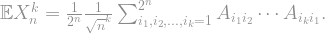
Given a matrix , it’s often very difficult to say something about a single, particular one of its eigenvalues. However, saying something about all of them is sometimes easy: the sum of all eigenvalues is just the trace of the matrix, i.e. the sum of its diagonal entries. Similarly, since has eigenvalues , the sum is given by the trace of the matrix . So all we need to do is calculate

What is this trace? If you carry out the the by-the-book matrix multiplication, you’ll see that every entry of consists of a sum of products of ‘s entries, where each product has “chasing indices”, i.e. it is of the form

In our case, this gives a massive sum:

That’s a lot of summands to sum over. But luckily, most of them are going to be 0. Remember, our matrix isn’t just any old matrix; it’s the adjacency matrix of a graph, so is if vertex is not connected to vertex . This clears out a lot of the summands — anything which contains a “non-edge” term will be and contribute nothing to the sum. In effect, this forces the sequence of indices to “walk” on the edges of the graph: you can think of the indices as the positions of an ant which starts at vertex and can traverse along the edges. For each starting position , the sum above then just counts the number of walks of length that the ant can take. Also, since we always have the term at the end, these walks have to return back to the point where they started, so in fact we are counting the number of back-to-origin walks.

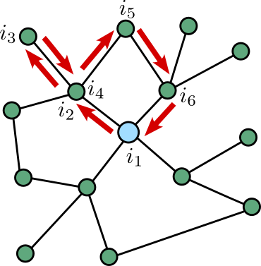
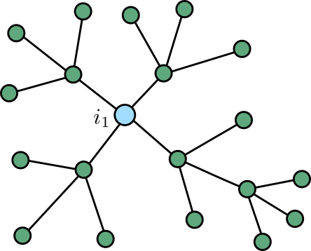
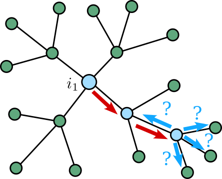
There is a whole art in counting the number of possible paths, but the simplest case is when you are walking on a graph that doesn’t have any cycles, i.e. a tree. Suppose that around your point of origin, the graph looks like a tree, i.e. at every step, you can branch out to different vertices, and unless you directly backtrack and undo the last step you took, you can never accidentally go back to the origin.

Suppose that at some point in time, the ant is already some distance away from the origin. For its next step, it generally has two options: it can either increase its distance from where it started, by taking one of the edges that lead away from it, or it can go back down towards its origin.

The fundamental observation is that, since the ant must end up back where it started, for each step that it walks away from the origin, it must, at some point, take a step back which brings it closer. This means that if the walk is of length , then it must make exactly steps that increase its distance, and steps which decrease its distance. (In particular, must be even!). Every time the ant increases its distance, there are either or edges it can walk along to do so (depending on whether it was at the origin or not), and every time the ant decreases its distance, there is only one edge it can go along. So, once the ant decides on which times it will increase the distance, and which times it will decrease them, there are only about different walks it can take.

So all that is left in order to count how large the sum above is, is to count in how many different ways the ant can choose a “hiking-plan” of when to increase the distance, and when to decrease the distance, keeping in mind that it must return to the origin after steps. If you have recurring nightmares from “Introduction to combinatorics”, you might recognize that this is exactly the Catalan numbers (which, as a fan of the Lisp programming language, I always remember as “the number of ways to write a block of well-balanced parentheses, e.g. “((()()))()”).

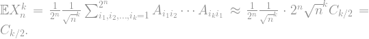
To summarize: if the graph around looks like a regular tree, then the number of all walks starting at will be about . And if this happens for almost every vertex in the graph, then

And — what do you know, who could have guessed it — if you do the math, the number is exactly what you get when you compute the (even) -th moment of , i.e. . So we get as needed!

Now, random regular graphs, despite their cordial manners, are not exactly trees: they do have some cycles in them. But as it turns out, they have so little of them, that this doesn’t really matter in the limit as .

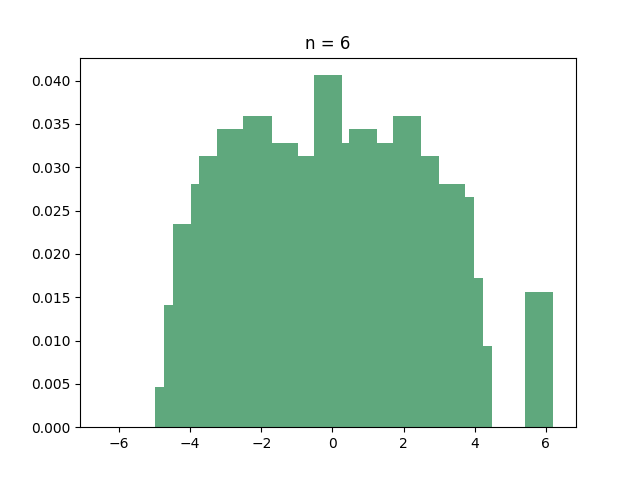
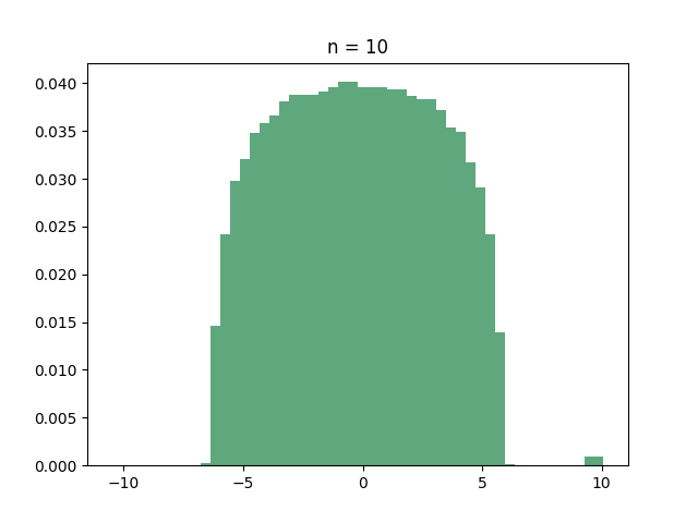
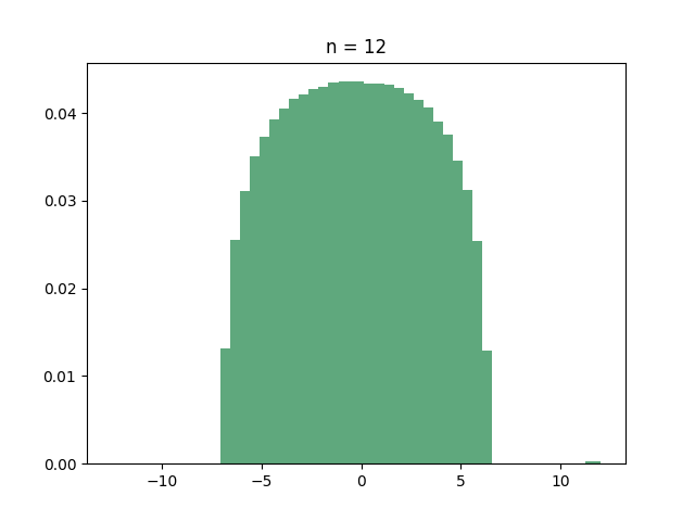
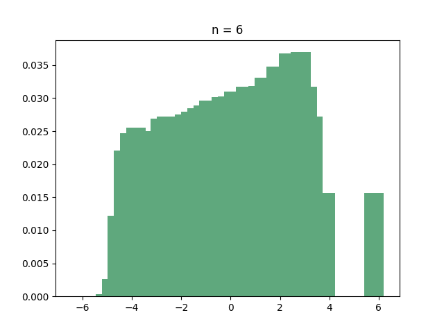
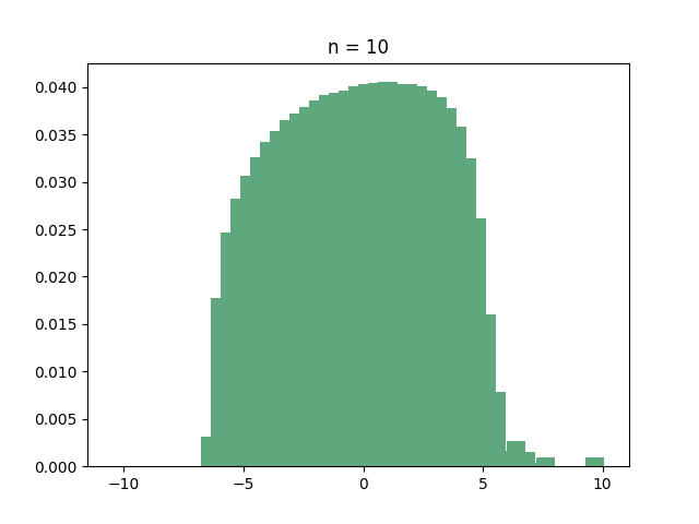
Back to business. We talked a lot about the eigenvalues of the hypercube (they converge to Gaussian) and the eigenvalues of random regular graphs (they converge to the semicircle). What about the duplicube?! As is tradition, we start with numerics. Here are the histograms of the eigenvalues of the random-matching duplicube:

If you are thinking, “This histogram looks like NEITHER the eigenvalues of the hypercube NOR the eigenvalues of the random regular graph. It must converge to something else!”, then you’d be wrong! Sorry about that.

Theorem: The distribution of the -normalized eigenvalues of the duplicube converges to the semicircle distribution.

In this sense, the duplicube is more like a random regular graph than the hypercube. The proof of the theorem follows the same outline as above: we used the moment method, and showed that while the duplicube does have cycles, there are not enough of them to change the combinatorics of Catalan-counting. However, it is probably quite true that there are more cycles in the duplicube than in random regular graphs, and this should mean that the convergence towards the semicircle law is slower (it takes more time for the “cycle effects” to die out).

What now?
Many questions remain — practically every question you can ask about other random graph models, you can ask about this one as well. We list about a dozen of them in our paper which we think might lead to interesting results + might not be too difficult to investigate. An important one, in my opinion, is that of derandomization: at every step of the duplimatching operation, instead of picking a uniformly random matching, can you pick a simple deterministic matching that gives you, say a graph with asymptotically smaller diameter than the hypercube?